Mini Project 4 – Math Stat Blog

“I have followed all rules for collaboration for this project, and I have not used generative AI on this project.”

The question of interest for this project is can we predict the probability that Nadal wins a point on his own serve against his primary rival, Novak Djokovic, at the French Open (the most prestigious clay court tournament in the world). We will answer this by using 3 different priors, a noninformative, and two informative priors based on preexisting knowledge or not. We will then update our posterior distributions to take into account the 2020 French open to get a more accurate estimate at the end, finishing off the project with 3 different credible posterior intervals with 90% confidence.

library(tidyverse)

── Attaching core tidyverse packages ──────────────────────── tidyverse 2.0.0 ──
✔ dplyr     1.1.4     ✔ readr     2.1.5
✔ forcats   1.0.0     ✔ stringr   1.5.1
✔ ggplot2   3.5.1     ✔ tibble    3.2.1
✔ lubridate 1.9.4     ✔ tidyr     1.3.1
✔ purrr     1.0.4     
── Conflicts ────────────────────────────────────────── tidyverse_conflicts() ──
✖ dplyr::filter() masks stats::filter()
✖ dplyr::lag()    masks stats::lag()
ℹ Use the conflicted package (<http://conflicted.r-lib.org/>) to force all conflicts to become errors

ps <- seq(0, 1, length.out = 1000)

noninformative_alpha <- 1
noninformative_beta <- 1

noninformative_prior <- dbeta(ps,
                              noninformative_alpha, noninformative_beta)

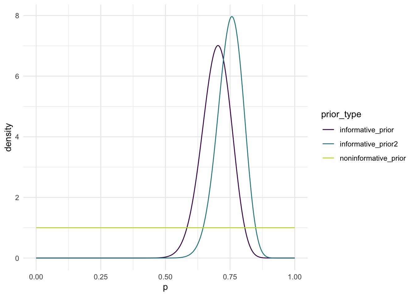
The fist prior is completely non-informative. This means we have no preexisting knowledge of Nadal’s performance or any idea of how it will go, so we will use a Beta(1, 1), which is equal to Uniform(0, 1) where 0 represents a loss and 1 represents a win on a serve. Uniform(0,1) assigns the same probability for every value in the interval, not making any assumptions about the points won on Nadal’s serves.

target_mean <- 0.697

alphas <- seq(0.1, 100, length.out = 500)
betas <- 0.303 * alphas / 0.697

param_df <- tibble(alphas, betas)
param_df <- param_df |> mutate(vars = 
                    (alphas * betas) / ((alphas + betas)^2 * (alphas + betas + 1)))


target_var <- 0.05657 ^2

param_df <- param_df |> mutate(dist_to_target = abs(vars - target_var))
param_df

# A tibble: 500 × 4
   alphas  betas   vars dist_to_target
    <dbl>  <dbl>  <dbl>          <dbl>
 1  0.1   0.0435 0.185          0.181 
 2  0.300 0.131  0.148          0.144 
 3  0.500 0.218  0.123          0.120 
 4  0.701 0.305  0.105          0.102 
 5  0.901 0.392  0.0921         0.0889
 6  1.10  0.479  0.0819         0.0787
 7  1.30  0.566  0.0737         0.0705
 8  1.50  0.653  0.0670         0.0638
 9  1.70  0.740  0.0614         0.0582
10  1.90  0.827  0.0566         0.0534
# ℹ 490 more rows

param_df |> filter(dist_to_target == min(dist_to_target))

# A tibble: 1 × 4
  alphas betas    vars dist_to_target
   <dbl> <dbl>   <dbl>          <dbl>
1   45.3  19.7 0.00320     0.00000310

informative_alpha <- 45.345
informative_beta <- 19.713

For the second prior, it is informative based on a clay-court match the two played in the previous year. In that match, Nadal won 46 out of 66 points on his own serve. The standard error of this estimate is 0.05657. Again, I chose a beta distribution but to find the alphas and betas I worked backwards from the mean equation for a beta distribution (E(x) = alpha/alpha+beta). Once I found Beta = (0.303 * alpha)/0.697, I assigned a sequence of values for alpha and used this formula to solve for beta. In addition to this, I also incorporated the standard error into a target variance, by squaring it and made sure the parameters were adjusted accordingly.

target_mean <- 0.75

alphas <- seq(0.1, 100, length.out = 500)
betas <- 0.25 * alphas / 0.75

param_df <- tibble(alphas, betas)
param_df <- param_df |> mutate(vars = 
                    (alphas * betas) / ((alphas + betas)^2 * (alphas + betas + 1)))


target_var <- 0.05 ^2

param_df <- param_df |> mutate(dist_to_target = abs(vars - target_var))
param_df

# A tibble: 500 × 4
   alphas  betas   vars dist_to_target
    <dbl>  <dbl>  <dbl>          <dbl>
 1  0.1   0.0333 0.165          0.163 
 2  0.300 0.100  0.134          0.131 
 3  0.500 0.167  0.112          0.110 
 4  0.701 0.234  0.0969         0.0944
 5  0.901 0.300  0.0852         0.0827
 6  1.10  0.367  0.0760         0.0735
 7  1.30  0.434  0.0686         0.0661
 8  1.50  0.500  0.0625         0.0600
 9  1.70  0.567  0.0574         0.0549
10  1.90  0.634  0.0530         0.0505
# ℹ 490 more rows

param_df |> filter(dist_to_target == min(dist_to_target))

# A tibble: 1 × 4
  alphas betas    vars dist_to_target
   <dbl> <dbl>   <dbl>          <dbl>
1   55.6  18.5 0.00250     0.00000246

informative_alpha2 <- 55.555
informative_beta2 <- 18.519

For the third prior, it is another informative one based on a sports announcer, who claims that they think Nadal wins about 75% of the points on his serve against Djokovic. They are also “almost sure” that Nadal wins no less than 70% of his points on serve against Djokovic. To figure out this final prior, I used the same strategy for the second prior with a little bit different logic. For this prior it will be another Beta, and we have once again been given the proportion of wins and can work backwards with the mean formula to get the betas = (0.25 * alphas) / 0.75. To make sure that this mean does not go below 70%, I chose a standard error of 0.05 and proceeded with the same strategy as the first prior.

informative_prior <- dbeta(ps, informative_alpha,
                           informative_beta)
informative_prior2 <- dbeta(ps, informative_alpha2,
                           informative_beta2)

noninformative_prior <- dbeta(ps,
                              noninformative_alpha, noninformative_beta)


prior_plot <- tibble(ps, informative_prior, noninformative_prior, informative_prior2) |>
  pivot_longer(2:4, names_to = "prior_type", values_to = "density")

ggplot(data = prior_plot, aes(x = ps, y = density, colour = prior_type)) +
  geom_line() +
  scale_colour_viridis_d(end = 0.9) +
  theme_minimal() +
  labs(x = "p")

informative_alpha_post <- informative_alpha + 56
informative_beta_post <- informative_beta + (84 - 56)
informative_post <- dbeta(ps, informative_alpha_post,
                          informative_beta_post)

#posterior mean for 2nd prior
informative_alpha_post / (informative_alpha_post + informative_beta_post)

[1] 0.6799031

informative_alpha_post2 <- informative_alpha2 + 56
informative_beta_post2 <- informative_beta2 + (84 - 56)
informative_post2 <- dbeta(ps, informative_alpha_post2,
                          informative_beta_post2)
#posterior mean for 3rd prior
informative_alpha_post2 / (informative_alpha_post2 + informative_beta_post2)

[1] 0.7057138

## CHANGE THESE
noninformative_alpha_post <- noninformative_alpha + 56
noninformative_beta_post <- noninformative_beta + (84 - 56)
noninformative_post <- dbeta(ps, noninformative_alpha_post,
                             noninformative_beta_post)
#posterior mean for noninformative prior
noninformative_alpha_post / (noninformative_alpha_post + noninformative_beta_post)

[1] 0.6627907

plot_df <- tibble(ps,
                     informative_post, noninformative_post, informative_post2) |>
  pivot_longer(2:4, names_to = "distribution", values_to = "density")

ggplot(data = plot_df, aes(x = ps, y = density, colour = distribution)) +
  geom_line() +
  scale_colour_viridis_d(end = 0.9) +
  theme_minimal() +
  labs(x = "p")

Credible Intervals

noninformative_post_int <- qbeta(c(0.05, 0.95), 57, 29)

informative_post_int <- qbeta(c(0.05, 0.95), informative_alpha + 56, informative_beta + (84 - 56))

informative_post_int2 <- qbeta(c(0.05, 0.95), informative_alpha2 + 56, informative_beta2 + (84 - 56))

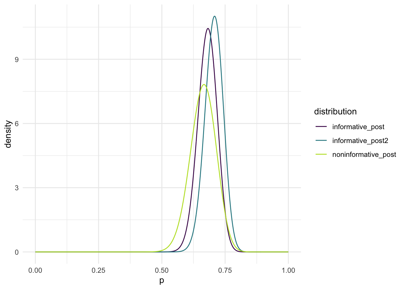
The three posteriors that I ended up with were all a little different from eachother. The noninformative prior gave the lowest posterior mean of 0.66279, followed by the posterior mean for the prior based on the previous year at 0.6768, then finally the highest mean of 0.6799 belongs to the prior based on the announcers estimate. They are all different from eachother slightly because of the information we used to obtain the priors. The non-informative prior is the closest to the actual mean from 2020, 0.6667. The variance of the non informative prior is the highest based on the plot of the posterior distributions. Between the two informative posteriors, the one based on the announcer’s prediction has a very slightly lower variance than the one based on data from the previous year, yet this is barely noticeable and at the end of the day they look like they have almost exactly the same variance. If I had to choose one posterior to rely on, I would choose the one based on the previous year’s data. There is too much variance within the non-informative posterior. Because the variances for the two informative posteriors are so similar, I won’t take that very strongly into consideration. Between the two, the one based on the previous years data has a posterior mean closer to the 2020 match, and I would pick that one.

In conclusion, I found that using an informative prior in this case helps make the estimates closer to the actual win percentage with a lower variance. There is a lot more variabliity in a non informative prior because you are assuming there is no difference between players skill level, which is never the case in these scenarios.